Attention
These pages are under construction — come back soon!
Doing everything automatically
The previous part computed one screening parameter via three calculations run by hand. This part computes one for every orbital of the same molecule, and both the ionization potential and the electron affinity that follow from them, in a single command.
The input file
Download ozone.yaml and place it in an empty directory. Here it
is in full:
# The ionization potential and electron affinity of ozone, with the KI
# functional and screening parameters computed from total-energy differences.

workflow:
  task: singlepoint               # spectral properties at fixed geometry
  correction: ki                  # the KI flavor of the correction, not KIPZ
  screening_method: dscf          # screening from total-energy differences
  init_orbitals: kohn-sham        # the orbitals the correction acts on
  alpha_numsteps: 1               # one pass of the screening-parameter loop
  pseudo_library: SG15/1.2/PBE/SR # scalar-relativistic, generated with PBE

atoms:
  cell_parameters:
    vectors:                      # a box of vacuum around the molecule
      - [8.1738, 0.0, 0.0]
      - [0.0, 6.0, 0.0]
      - [0.0, 0.0, 6.66]
    units: angstrom
    periodic: false               # an isolated molecule, not a crystal
  atomic_positions:
    units: angstrom
    positions:                    # bent, with 1.27 Å bonds and a 117° angle
      - [O, 4.0869, 3.0, 2.89]
      - [O, 5.1738, 3.0, 3.55]
      - [O, 3.0, 3.0, 3.55]

calculator_parameters:
  ecutwfc: 50.0                   # wavefunction cutoff (Ry)
  nbnd: 10                        # 9 filled orbitals, plus 1 empty for the LUMO
Warning
The cell and cutoffs in this file are deliberately rough, so that the whole workflow finishes in minutes. They are not converged! Use this file to learn the input format, not as something to copy-paste for production work.
The workflow block describes the workflow that will be run.
screening_method: dscf # screening from total-energy differences
selects the procedure you carried out by hand: constrained calculations at \(N\), \(N-1\) or \(N+1\) electrons, whose energy differences are compared against the orbital energies (see the theory page).
init_orbitals: kohn-sham # the orbitals the correction acts on
uses the Kohn-Sham orbitals as the variational orbitals — what the hand copies of the
.dat files achieved in the previous part. This is common practice for molecules;
periodic systems use Wannier functions instead.
alpha_numsteps: 1 # one pass of the screening-parameter loop
computes the screening parameters once, from a guess, and uses them. Increasing this number will refine them self-consistently.
pseudo_library: SG15/1.2/PBE/SR # scalar-relativistic, generated with PBE
determines that PBE will be the base functional that the KI correction is applied on top of.
The atoms block describes the cell and the atoms in it, much like a Quantum ESPRESSO
input file. The positions are Cartesian, in the units the block declares.
Question
Why is the simulation cell so much larger than the molecule itself?
Show answer
The cell is a box of vacuum that keeps the molecule’s periodic images apart (a plane-wave code works in a supercell even when the system is treated as non-periodic). Vacuum padding matters more here than in a ground-state calculation, because the screening calculations give the molecule a net charge and charged images interact via a long-ranged Coulomb tail. To compensate for this, the code will also apply a counter-charge correction that compensates the residual interaction between images, and these corrections have less to do the further apart the images are.
The calculator_parameters block holds other calculator settings.
nbnd: 10 # 9 filled orbitals, plus 1 empty for the LUMO
adds one empty orbital to the nine that ozone’s 18 valence electrons fill, which we need because the electron affinity is the energy of the LUMO. In later tutorials we will go into more detail on how to specify code-specific parameters.
Running the calculation
Warning
Make sure you have installed koopmans: see here for more details.
Of all the Quantum ESPRESSO codes, this workflow only needs kcp.x.
Run the calculation with
$ koopmans run ozone.yaml
The terminal shows a live progress table that grows as the workflow proceeds. At the end it reads
 Step                                                                      Status
 Koopmans DSCF Workflow                                                  finished
   DFT Init (nspin=1)                                                    finished
   DFT Init (nspin=2; dummy)                                             finished
   DFT Init (nspin=2)                                                    finished
   Compute Screening Parameters                                          finished
     Iteration 1                                                         finished
       KI Trial                                                          finished
       Compute Orbital Screening Parameters                              finished
         Compute Alpha Orb 1                                             finished
           DFT N-1                                                       finished
         Compute Alpha Orb 2                                             finished
           DFT N-1                                                       finished
         ...
         Compute Alpha Orb 9                                             finished
           DFT N-1                                                       finished
         Compute Alpha Orb 10                                            finished
           DFT N+1 Dummy                                                 finished
           PZ Print                                                      finished
           DFT N+1                                                       finished
   Run Final KI                                                          finished
     KI Final                                                            finished

Workflow completed successfully!
Reading it top to bottom, we can identify three stages of the workflow:
Initialization (DFT Init)
This is the PBE calculation you ran first by hand, with one wrinkle: it takes three steps rather than one. Adding and removing single electrons later on requires a spin-resolved description, so the workflow must end up at a spin-resolved calculation — but it gets there via a detour, running a spin-unpolarized calculation, then a dummy spin-resolved one that lays out the restart files, and finally a spin-resolved calculation that restarts from the spin-unpolarized density duplicated into both spin channels.
Question
Why the detour, instead of one spin-resolved calculation from scratch?
Show answer
For ozone — a closed-shell molecule — a direct spin-resolved calculation would in fact converge to the correct spin-symmetric solution. The detour has two virtues all the same. In harder systems, a spin-resolved calculation started from scratch can collapse into a spurious broken-symmetry solution with \(n^\uparrow(\mathbf{r}) \neq n^\downarrow(\mathbf{r})\); handing it an already-converged symmetric density avoids that. And it is cheaper: most of the self-consistency cycles happen in the spin-unpolarized problem, which has half the wavefunctions.
From this point on the density never changes: KI, by construction, returns the same density as its base functional. (This is not true of KIPZ.)
Screening parameters (Compute Screening Parameters)
This is the bulk of the calculation, and it is the trial-KI-and-constrained-DFT pair from the previous part, repeated for every orbital instead of just the HOMO:
the
KI trialstep plays the role of your trial run, with the guess \(\alpha_i = 0.6\) in place of 0.7 and every orbital’s energy recorded rather than the HOMO’s alone;then, for each of the nine filled orbitals in turn, a constrained \(N-1\) calculation like the one you ran, with
fixed_bandpointing at that orbital;the one empty orbital runs the procedure in reverse — two preparatory calculations followed by an \(N+1\)-electron constrained calculation in which the orbital is filled, giving \(E_i(N+1)\).
Each orbital’s screening parameter then comes from the formula you derived, applied to
that orbital’s own energies. With alpha_numsteps: 1, the loop stops there.
The final calculation (Run Final KI)
Your ozone_ki_opt.in run, with ten different screening parameters in place of one
applied universally. The orbital energies it prints are the spectral properties we are
after.
The outputs
The results land in a directory named after the input file — here ozone/ — laid out
to mirror the workflow outline above:
ozone
├── 01-count_electrons_task
│   └── inputs
├── 02-dft_init_nspin1
│   ├── inputs
│   └── outputs
├── 03-dft_init_nspin2_dummy
│   ├── inputs
│   └── outputs
├── 04-dft_init_nspin2
│   ├── inputs
│   └── outputs
├── 05-ComputeScreeningParameters
│   └── 01-ScreeningIteration
│       ├── 01-ki_trial
│       │   ├── inputs
│       │   └── outputs
│       └── 02-compute_orbital_screening_parameters
│           ├── 01-compute_alpha_orb_1
│           │   ├── 01-dft_n_minus_1
│           │   └── 02-compute_alpha_from_dscf
│           ├── ...
│           └── 10-compute_alpha_orb_10
│               ├── 01-dft_n_plus_1_dummy
│               ├── 02-pz_print
│               ├── 03-dft_n_plus_1
│               └── 04-compute_alpha_from_dscf
├── 06-RunFinalKI
│   ├── inputs
│   └── outputs
└── README
One directory per step, numbered in the order the steps ran. A step that is a Quantum
ESPRESSO calculation holds the exact input file the engine generated (aiida.cpi)
plus its pseudopotentials in inputs/, and everything the calculation wrote
(aiida.cpo and more) in outputs/.
Note
The engine also keeps its own complete record of every calculation in its database —
that is how an interrupted workflow resumes where it left off, and how a repeated
calculation is served from cache instead of running twice. The ozone/ directory
is a plain-file export of that record for you to read.
Interpreting the results
You read the ionization potential off a kcp.x output once already; this time the
electron affinity comes with it, as the negative of the LUMO energy. Open
ozone/06-RunFinalKI/outputs/aiida.cpo and search near the bottom for the HOMO
Eigenvalue and LUMO Eigenvalue lines — and, for the PBE comparison, find the same
lines in the initialization output, ozone/04-dft_init_nspin2/outputs/aiida.cpo.
Question
What do you find?
Show answer
Near the bottom of the final KI output:
HOMO Eigenvalue (eV)
-12.4945
LUMO Eigenvalue (eV)
-1.7184
Electronic Gap (eV) = 10.7761
Eigenvalues (eV), kp = 1 , spin = 1
-40.3490 -33.0412 -24.3772 -19.7139 -19.5385 -19.2977 -13.5960 -12.7467 -12.4945
Empty States Eigenvalues (eV), kp = 1 , spin = 1
-1.7184
The initialization output puts the PBE HOMO at −7.9229 eV and the PBE LUMO at −6.1058 eV.
KI puts the ionization potential at 12.49 eV and the electron affinity at 1.72 eV, where PBE would have given 7.92 eV and 6.11 eV. This is the same 12.49 eV the previous part arrived at by hand, as it should be: the screening parameter computed there enforces the same Koopmans condition on the same orbital.
An orbital energy is a vertical removal energy — the geometry does not relax with the electron — so the measurement to compare against is vertical photoemission, which puts ozone’s first ionization at 12.73 eV [36]. KI is a quarter of an electronvolt below that; PBE is nearly five below. The measured electron affinity is 2.10 eV, which KI undershoots by 0.4 eV and PBE overshoots by four.
Note
Tables of ozone’s properties usually quote an ionization energy of 12.52 eV. That is the adiabatic value, which lets the ion relax into its own geometry and so comes out lower. Orbital energies correspond to vertical ones.
Photoemission resolves more than the frontier orbital, and KI predicts a binding energy
for every occupied one. The three outermost are cleanly assigned — 12.73, 13.00 and
13.54 eV [36] — while the deeper assignments are less certain, so they
are left out. The three KI values sit at the end of the final KI output’s
Eigenvalues line, and the PBE ones in the corresponding line of the initialization
output. Plotting one against the other:
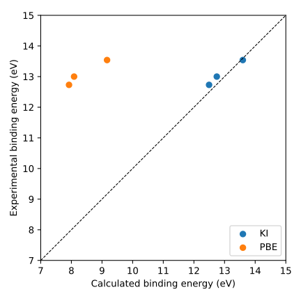
Calculated against experimental binding energies for the three outermost occupied
orbitals of ozone, from this run; a point on the dashed line agrees perfectly with
experiment. Made by plot_ozone_spectrum.py,
which reads the two Eigenvalues lines out of the ozone/ directory.
KI lands within about a quarter of an electronvolt of experiment for all three orbitals; PBE misses by more than four.
The screening parameters behind this result are recorded in the final calculation’s
input: ozone/06-RunFinalKI/inputs/file_alpharef.txt lists one \(\alpha_i\) per
orbital, here ranging from 0.66 to 0.79 — each one computed, not fitted.
Question
Why one screening parameter per orbital, rather than the single α of the previous part?
Show answer
The single \(\alpha\) you computed enforces the Koopmans condition on the HOMO alone — which is why the ionization potential came out right there, and why nothing else did. In particular the electron affinity suffers, because an \(\alpha\) tuned for the HOMO cannot simultaneously describe the LUMO. Screening is an orbital-by-orbital affair.
Question
What happens if you increase alpha_numsteps to 2 and rerun?
Show answer
With alpha_numsteps: 1 the screening parameters are computed once from the
starting guess and never checked for self-consistency. With a second step, the
workflow repeats the screening loop starting from the just-computed parameters
instead of 0.6, and only updates a parameter further if its residual is above the
convergence threshold (alpha_conv_thr). You should find that the parameters
barely move — the first pass already brought them close to self-consistency.
From python
The same calculation runs from python, which is the easier route for sweeping a parameter or working in a notebook. Reading the input file and running it are a line each, and the results come back as a dict instead of as output files to search:
from koopmans import read_input_file, run

results = run(read_input_file("ozone.yaml"))

homo = results["parameters"]["homo_energy"]
lumo = results["parameters"]["lumo_energy"]

print(f"IP = {-homo:.2f} eV")  # IP = 12.49 eV
print(f"EA = {-lumo:.2f} eV")  # EA = 1.72 eV
Energies are in eV, and the ionization potential and electron affinity are the negated
HOMO and LUMO energies as before — the same two numbers read out of aiida.cpo above.
results carries the rest of the final calculation’s outputs alongside them,
eigenvalues among them.
run blocks python until the workflow finishes. For a calculation long enough that
this is inconvenient, the alternative is submit, which returns an integer ID
immediately and leaves the workflow running in the background. Later, use
outputs(<ID>) to read the finished result. See Calling within python for more detail.